1. Problem
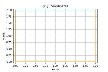
$0 < x < 2$ $0 < y < 2$인 정사각형 영역에서 Laplace equation을 만족하는 $u(x,y)$에 대하여 다음과 같은 boundary condition을 만족한다고 하자.
Boundary condition:
- $x=0 \rightarrow u=0$
- $x=2 \rightarrow u=0$
- $y=0 \rightarrow u=0$
- $y=2 \rightarrow u=f(x)$ where $f(x)=\sin\frac{\pi x}{2}$
2. Analytical Solution
2.1 Separation of Variables
\(u(x,y) = X(x)Y(y) \tag{3}\)
$X(x)Y(y)$를 $(2)$에 대입하면
\[Y(y)\frac{d^{2}X(x)}{d x^{2}} + X(x)\frac{d^{2}Y(y)}{d y^{2}} = 0 \tag{4}\]$(4)$의 양변을 $(3)$으로 나누어주면
\[\frac{1}{X(x)}\frac{d^{2}X(x)}{d x^{2}} = - \frac{1}{Y(y)}\frac{d^{2}Y(y)}{d y^{2}} = -k^{2} = const. \tag{5}\]where $k>0$.
\[\therefore X(x) = A\sin kx +B\cos kx \quad Y(y) = Ce^{ky} + De^{-ky} \tag{6}\]2.2 Boundary Condition 1
Boundary Condition 1에 의해 $u(x=0, y) = X(x=0)Y(y) = 0$을 $y$에 상관없이 만족해야 하므로
\[\therefore X(x)=A\sin kx \tag{7}\]2.3 Boundary Condition 2
Boundary Condition 2에 의해 $u(x=2, y) = X(x=2)Y(y) = 0$을 $y$에 상관없이 만족해야 하므로 $X(x=2)=A\sin{2k}=0$이 성립한다.
\[\therefore k = \frac{n\pi}{2} \ (n = 1, 2, 3, \ldots) \tag{8}\]$(6), (7), (8)$을 $(3)$에 대입하면
\[u_{n}(x,y)=(C_{n}e^{\frac{n\pi}{2}y} + D_{n}e^{-\frac{n\pi}{2}y})\sin{\frac{n\pi}{2}x} \tag{9}\]2.4 Boundary Condition 3
Boundary Condition 3에 의해 $u_{n}(x,y=0) = (C_{n} + D_{n})\sin{\frac{n\pi}{2}x} = 0$을 $x$에 상관없이 만족해야 하므로 $C_{n} + D_{n} = 0$이 성립한다.
\[\therefore D_{n} = - C_{n} \tag{10}\] \[\therefore u_{n}(x,y)=C_{n}(e^{\frac{n\pi}{2}y} - e^{-\frac{n\pi}{2}y})\sin{\frac{n\pi}{2}x} \tag{11}\]미분 연산은 linear하고 따라서 Laplacian $\nabla^{2}$도 linear한 operation이므로 Laplace equation $(1)$을 만족하는 general solution $u(x,y) = \sum_{n=1}^{\infty} u_{n}(x,y)$는 다음과 같이 쓸 수 있다.
\[u(x,y) = \sum_{n=1}^{\infty} C_{n}(e^{\frac{n\pi}{2}y} - e^{-\frac{n\pi}{2}y})\sin{\frac{n\pi}{2}x} \tag{12}\]2.5 Boundary Condition 4: Fourier Series
Boundary Condition 4에 의해 $u(x,y=2) = f(x) = \sin{\frac{\pi x}{2}}$를 만족해야 하므로
\[u(x,y=2) = \sum_{n=1}^{\infty} C_{n}(e^{n\pi} - e^{-n\pi})\sin{\frac{n\pi}{2}x} = \sin{\frac{\pi x}{2}} \tag{13}\]Let $c_{n} = C_{n}(e^{n\pi} - e^{-n\pi})$ and $(13)$ will be a Fourier series form with period $l = 2$.
\[\therefore u(x,2) = \sum_{n=1}^{\infty} c_{n}\sin{\frac{n\pi}{2}x} = \sin{\frac{\pi x}{2}} \tag{14}\]where $u(x,2)$ is a function of $x$.
Fourier series에 의하여 $c_{n} = \frac{2}{l} \int_{0}^{l} f(x)\sin{\frac{n\pi}{l}x}dx = \int_{0}^{2} \sin{\frac{\pi x}{2}}\sin{\frac{n\pi}{l}x}dx = 0 \ (n \neq 1)$.
\[\therefore C_{n}=0 \ (n \neq 1) \tag{15}\]For $n=1$, $c_1 = \frac{2}{l} \int_{0}^{l} f(x)\sin{\frac{\pi}{l}x}dx = \int_{0}^{2} \sin^{2}{\frac{\pi}{2}x}dx = 0$.
\[\therefore C_1 = \frac{1}{e^{\pi} - e^{-\pi}} \tag{16}\]2.6 Solution
$(12)$와 $(15), (16)$에 의하여
\[\therefore u(x,y) = \frac{1}{e^{\pi} - e^{-\pi}}(e^{\frac{\pi}{2}y} - e^{-\frac{\pi}{2}y})\sin{\frac{\pi}{2}x} \tag{17}\]3. Numerical Solution
Let’s solve numerically above problem and draw graphs using Python library numpy and matplotlib.
3.1 What is Lattice Laplacian?
미적분 시간에 배웠던 리만 합과 비슷하다.
그래프를 연속적인 선 또는 면으로 생각하지 않고 잘게 조각내어 (Lattice) 각 조각에 대해 계산을 하는 것이다.
당연히 조각의 수가 클수록 계산 결과는 참 값에 가까워 진다.
여기서는 단지 조각을 나누는 것을 Laplacian을 계산하는데 사용하는 것 뿐이다.
3.2 Basic Settings
I used Jupyter Notebook.
1
2
3
import math, random
import numpy as np
from matplotlib import pyplot as plt
1
2
3
4
5
N = 100                         # divide area into N equal parts
e = [10 ** i for i in range(5)] # epoch

x_left, x_right = 0, 2          # x coordinates 0 < x < 2
y_left, y_right = 0, 2          # y coordinates 0 < y < 2
영역을 $x$축 방향으로 N만큼 $y$축 방향으로 N만큼 동일한 크기의 블럭으로 나눌 것이다. 따라서 총 N$^{2}$개의 블럭이 생긴다. N = 100이므로 영역을 총 10000개의 동일한 크기의 블럭으로 나누게 된다. 각각의 블럭에는 하나의 실수값이 배치된다.
1
2
3
4
5
6
7
8
9
10
11
12
13
14
def boundary_f(j):
    return math.sin(math.pi * j / (N-1)) if j != N-1 else 0

def Lattice(coor, i, j):
    return (coor[i+1,j] + coor[i-1,j] + coor[i,j+1] + coor[i,j-1]) / 4

def to_matrix(maths):
    return maths * (N-1) / 2

def to_maths(matrix_idx):
    return matrix_idx * 2 / (N-1)
'''
to_matrix and to_maths are used to transform two different scales.
'''
3.3 Coordinates Initialisation
Boundary Condition 1, 2, 3에 의하여 $x \times y = 0$ or $x = 2$일 때 $u = 0$이다.
1
2
3
4
5
coordinates = np.matrix([
    [ 0 if i * j == 0 or j == 99 else random.random()
    for j in range(N) ] for i in range(N)])
print(coordinates)
print(np.shape(coordinates))
1
2
3
4
5
6
7
8
9
10
>>>
[[0.      0.         0.         ... 0.         0.         0.       ]
 [0.      0.76647573 0.85497858 ... 0.65825655 0.70332986 0.       ]
 [0.      0.08536608 0.15863341 ... 0.76746172 0.06642089 0.       ]
 ...
 [0.      0.01348908 0.74033728 ... 0.67932431 0.25610339 0.       ]
 [0.      0.26472592 0.4982553  ... 0.67932193 0.82749659 0.       ]
 [0.      0.37740627 0.06626904 ... 0.33949001 0.65761649 0.       ]]

 (100, 100)
$(i,j)$ coordinates 행렬의 $(0,0) \ldots (99,99)$에 boundary condition에 맞는 $u(i,j)$ 값들을 대입한 결과이다. 첫번째 행과 열의 index는 0부터 시작한다고 한다. 이때 $(i=0, j)$는 $y=0 \ \text{(x-axis)}$이고 $(i, j=0)$, $(i, j=0)$는 각각 $x=0 \ \text{(y-axis)}$, $x=2$이다. 좌우는 동일하고 상하는 대칭이라고 생각하면 쉽다.
경계가 아닌 영역의 값들은 random.random 함수를 이용해 임의로 설정하였다. random.random 함수의 범위는 $[0,1)$이다.
1
2
3
4
5
for j in range(N):
    coordinates[N-1,j] = boundary_f(j)

print(coordinates)
print(np.shape(coordinates))
1
2
3
4
5
6
7
8
9
10
>>>
[[0.      0.         0.         ... 0.         0.         0.       ]
 [0.      0.76647573 0.85497858 ... 0.65825655 0.70332986 0.       ]
 [0.      0.08536608 0.15863341 ... 0.76746172 0.06642089 0.       ]
 ...
 [0.      0.01348908 0.74033728 ... 0.67932431 0.25610339 0.       ]
 [0.      0.26472592 0.4982553  ... 0.67932193 0.82749659 0.       ]
 [0.      0.03172793 0.06342392 ... 0.06342392 0.03172793 0.       ]]

(100, 100)
99행$(i, j=99)$의 값들은 Boundary Condition 4에 맞게 초기화 되었다. 이제 경계값들을 모두 초기화 하였으므로 Lattice Laplacian 방법을 사용하여 영역 내부의 값들을 Laplace equation의 해가 되도록 계산할 것이다.
3.4 Lattice Laplacian
1
2
3
4
5
6
7
8
for iteration in range(M[4]): # M[4] == 10000
    updated = coordinates.copy()
    for i in range(1,N-1):
        for j in range(1,N-1):
            updated[i,j] = Lattice(coordinates, i, j) # main algorithm
    coordinates = updated.copy()

print(coordinates)
Lattice Laplacian 방법으로 계산하기 위해 Lattice 함수가 사용되었다.
1
2
3
4
5
6
7
8
9
10
11
12
13
14
>>>
[[0.00000000e+00 0.00000000e+00 0.00000000e+00 ... 0.00000000e+00
  0.00000000e+00 0.00000000e+00]
 [0.00000000e+00 9.05149261e-05 1.80482124e-04 ... 1.80938235e-04
  9.02863769e-05 0.00000000e+00]
 [0.00000000e+00 1.80657748e-04 3.62046303e-04 ... 3.61133027e-04
  1.81113859e-04 0.00000000e+00]
 ...
 [0.00000000e+00 2.97760537e-02 5.95212127e-02 ... 5.95221245e-02
  2.97755968e-02 0.00000000e+00]
 [0.00000000e+00 3.07362940e-02 6.14420957e-02 ... 6.14416388e-02
  3.07365222e-02 0.00000000e+00]
 [0.00000000e+00 3.17279335e-02 6.34239197e-02 ... 6.34239197e-02
  3.17279335e-02 0.00000000e+00]]
3.5 Comparison
이제 Lattice Laplacian 방법으로 계산한 numerical solution과 analytical solution을 비교해보자. 해는 2차원이므로 한눈에 보기위해 $y=x$ 상의 대각성분만 비교한다.
1
2
3
# diagonal components of numerical solution
numerical_D = [ coordinates[k,k] for k in range(N) ]
print(numerical_D)
1
2
>>>
[0.0, 9.051492612165759e-05, 0.00036204630303846545, 0.0008145536264188748, 0.0014479683888704415, 0.002262192578925126, 0.0032570965781172296, 0.004432516454671923, 0.0057882506519266064, 0.007324056069232347, 0.009039643532732965, 0.010934672653099383, 0.013008746067011209, 0.015261403058930425, 0.017692112559508054, 0.02030026551680779, 0.023085166636425375, 0.026046025486532558, 0.02918194696388458, 0.032491921116903445, 0.035974812322090176, 0.03962934781023135, 0.04345410553915224, 0.04744750141013394, 0.05160777582555922, 0.05593297958588381, 0.060420959124650356, 0.06506934108097397, 0.069875516209734, 0.07483662263061025, 0.07994952841810309, 0.085210813535783, 0.09061675111922281, 0.09616328811338223, 0.10184602527163852, 0.10766019652519125, 0.11360064773321746, 0.1196618148259129, 0.12583770135443223, 0.132121855463733, 0.13850734630643857, 0.14498673991806288, 0.15155207457628878, 0.158194835669457, 0.16490593010201152, 0.17167566026735373, 0.17849369762138528, 0.18534905589296713, 0.19223006397058925, 0.1991243385077322, 0.20601875629270433, 0.21289942643216264, 0.21975166240105992, 0.22655995401541534, 0.23330793938806976, 0.23997837693146368, 0.24655311747546033, 0.2530130765723304, 0.25933820706520894, 0.265507472000634, 0.27149881797017145, 0.27728914897062185, 0.2828543008768861, 0.2881690166262365, 0.29320692221749056, 0.29794050363341684, 0.30234108479960475, 0.306378806698003, 0.3100226077583663, 0.31324020565593985, 0.3159980806488562, 0.31826146059390104, 0.3199943077845279, 0.32115930776025226, 0.32171786024182647, 0.3216300723518796, 0.3208547542859944, 0.31934941760447066, 0.31707027632029117, 0.3139722509640386, 0.31000897581171327, 0.30513280946654564, 0.299294848990984, 0.2924449477900469, 0.28453173745214794, 0.27550265375831606, 0.26530396707543297, 0.2538808173536666, 0.2411772539526924, 0.2271362805255342, 0.21169990519290705, 0.19480919624479515, 0.17640434360961552, 0.15642472633469295, 0.13480898632487665, 0.11149510858894163, 0.08642050824591851, 0.05952212454565295, 0.03073652215969229, 0.0]
1
2
3
# diagonal curve of analytical solution
def analytical_curve(x) :
    return (1 / (math.exp(math.pi) - math.exp(-math.pi))) * (math.exp(math.pi * x / 2) - math.exp(-math.pi * x / 2) ) * math.sin(math.pi * x / 2)
same as
\[u(x,y=x) = \frac{1}{e^\pi - e^{-\pi}} (e^{\frac{\pi}{2}x} - e^{-\frac{\pi}{2}x}) \sin{\frac{\pi}{2}x} \tag{18}\]1
2
3
# diagonal components of analytical solution
analytical_D = [analytical_curve(to_maths(i)) for i in range(N)]
print(analytical_D)
여기서 range(N) = [0, 1, 2, 3, …, N] scale을 $0 < x < 2$ or $0 < y < 2$ scale로 변환하기 위해 to_maths 함수가 사용되었다.
1
2
>>>
[0.0, 8.719564034953965e-05, 0.000348782502451089, 0.0007847600557810537, 0.0013951262371926453, 0.0021798756825077846, 0.003138997250757162, 0.004272470841091858, 0.005580263502413895, 0.007062324835809864, 0.008718581689924405, 0.010548932149481523, 0.012553238817254581, 0.014731321389902822, 0.01708294852823681, 0.01960782902264963, 0.022305602254658084, 0.02517582795574172, 0.02821797526494911, 0.03143141108706486, 0.03481538775349818, 0.038369029988469715, 0.04209132118353773, 0.04598108898402343, 0.050036990191468796, 0.05425749498689222, 0.05864087048030098, 0.06318516359267706, 0.06788818327747664, 0.07274748208957724, 0.07776033711057267, 0.08292373024035567, 0.08823432786604633, 0.09368845992052209, 0.09928209834408527, 0.10501083496416883, 0.1108698588094348, 0.11685393287615993, 0.12295737036643943, 0.12917401041946688, 0.13549719335897334, 0.1419197354818319, 0.14843390341485826, 0.1550313880689629, 0.16170327822203961, 0.16844003376431332, 0.1752314586423092, 0.18206667354015907, 0.1889340883396197, 0.19582137440295191, 0.20271543672568848, 0.20960238600931966, 0.2164675107070291, 0.22329524909883774, 0.2300691614558475, 0.23677190235672393, 0.2433851932231207, 0.24988979514441964, 0.25626548206594685, 0.26249101441871997, 0.2685441132727842, 0.2744014351003073, 0.28003854723881805, 0.2854299041492907, 0.2905488245681944, 0.2953674696571421, 0.29985682225837657, 0.303986667369028, 0.30772557395185623, 0.31104087820504595, 0.31389866841855957, 0.31626377154954427, 0.3180997416543604, 0.31936885031990225, 0.3200320792420534, 0.3200491151043135, 0.3193783469148662, 0.3179768659656088, 0.3158004685819258, 0.3128036618372501, 0.3089396724117084, 0.3041604587793692, 0.2984167269138126, 0.2916579497068696, 0.2838323903004722, 0.27488712953653843, 0.26476809773473436, 0.25342011101273926, 0.2407869123683057, 0.22681121774692625, 0.2114347673232622, 0.19459838222865572, 0.17624202696100233, 0.156304877716977, 0.13472539689009128, 0.11144141398123564, 0.08639021317126809, 0.05950862780776092, 0.030733142060230534, 1.2246467991473532e-16]
이제 그래프를 그려서 눈으로 비교해보자.
1
2
3
4
5
6
7
plt.plot(range(N), numerical_D, color='blue', label='numerical solution')
plt.plot(range(N), analytical_D, color='orange', label='analytical solution')
plt.xlabel("y == x")
plt.ylabel("u(x,x)")
plt.title("Iteration = 10000")
plt.legend(loc=2)
plt.show()

파란색 그래프가 주황색 그래프에 잘 근사되었음을 알 수 있다.
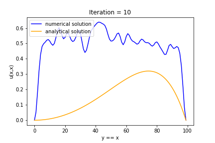
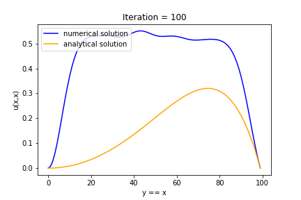
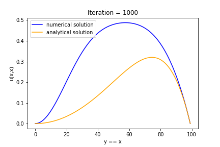
3.6 Graph by Iteration
Iteration = 10, 100, 1000, 10000 일 때의 각각의 그래프이다. Iteration 횟수가 증가함에 따라 analytical solution에 점점 다가가는 것을 볼 수 있다.